Your customers have a lot in common. They all like your brand and enjoy your products, and a lot of them are wearing your fashion right now. But your customers aren’t a single uniform group. They’re human beings, each with their own thoughts and feelings, and they want to be treated as such.
This is one of retail’s great problems right now. How do you take the store experience – one that’s inherently not individualized – and make each customer feel as though it’s been customized just for them?
Many retailers have tried to solve this problem through technology, like AI installations and iPad-armed store associates ready to make recommendations based on your purchase history. Notably, One retailer recently launched a series of pop-ups in an attempt to localize its assortments. But these are expensive and cumbersome strategies that merely add on to the one-size-fits-all store concept. A better way to make your stores feel more personalized is by tailoring your assortments to each location’s customer demand.
See also: Creative Marketing for Permanent Markdowns is a Band-Aid Solution
There are two sides to customer demand. First is raw demand, i.e. how many customers want to buy how many things. We frequently see this represented by sales volume. You probably already have a good idea of which stores perform best and worst based on sales.
Second is customer preference, i.e. how many customers prefer certain styles over others. You probably have an idea of your customers’ preferences by location as well. Certain stores might be more likely to sell fashion items than basics, and vice-versa. Even two stores that perform similarly in terms of sales volume will have distinct customer preferences. Customers in some locations might skew more toward casual items, and others more toward trendy pieces.
By combining these aspects of customer demand together, you can begin to create an accurate picture of what your customers want, by location.
Start by grouping your stores based on sales volume. But don’t fall into the trap of using overall sales volume as your retail store clustering method. Instead, look at sales volume by location at a product level. If a top store performs poorly when it comes to accessories, it shouldn’t be treated as a top store when it comes to accessories.
See also: Is Sales Volume The Right Metric For Retail Store Clustering?
Next, create additional groups of stores based on their customers’ unique preferences. These could be related to channel, country, currency, climate, or anything that they have in common.
Then, use these two types of clusters together to layer and tailor your buys.
Let’s use boots as an example.
Let’s say you have 250 stores in your chain, and your clusters show that when it comes to boots, you have 4 A stores, 59 B stores, 108 C stores, and 79 D stores. Relative to the most common store, your A stores can sell 2.20x as many boots, your B stores can sell 1.32x as many, your C stores can sell 1.00x as many, and your D stores can sell just 0.70x as many.
| Cluster | A | B | C | D |
|---|---|---|---|---|
| Store Count | 4 | 59 | 108 | 79 |
| Index | 2.20 | 1.32 | 1.00 | 0.70 |
Now, let’s say that your most common store can sell 8 pairs of a style of boots.
| Cluster | A | B | C | D | Total |
|---|---|---|---|---|---|
| Store Count | 4 | 59 | 108 | 79 | |
| Index | 2.20 | 1.32 | 1.00 | 0.70 | |
| Units per store | 17.6 | 10.56 | 8 | 5.6 | |
| Total buy quantity | 70 | 623 | 864 | 442 | 1,999 |
Using your clusters’ ability to sell this style of boots, you can calculate that you need 1,999 units to match customer demand.
But let’s say you want to exclude this style from your D stores. Even though you have 79 D stores and your most common store can sell 8 pairs, reducing your buy by 632 (79 stores x 8 units) units would take away more inventory than needed. As you can see from the table above, your D stores sell less than the most common store, so you can preserve inventory for your other locations (ensuring they’ll have enough product to satisfy demand) by only reducing your buy by 442 units.
| Cluster | A | B | C | D | Total |
|---|---|---|---|---|---|
| Store Count | 4 | 59 | 108 | 79 | |
| Index | 2.20 | 1.32 | 1.00 | 0.70 | |
| Units per store | 17.6 | 10.56 | 8 | 0 | |
| Total buy quantity | 70 | 623 | 864 | 0 | 1,557 |
Now that you’ve calculated your buy based on sales volume at a product class level, you can take this a step further by selecting which groups of stores should receive this buy based on customer preferences.
Let’s look at an example using to see how selecting stores by climate affects your buy.
| Cluster | A | B | C | D |
|---|---|---|---|---|
| Hot climate stores | 1 | 18 | 20 | 24 |
| Moderate climate stores | 2 | 30 | 56 | 15 |
| Cold climate stores | 1 | 11 | 32 | 40 |
| Total | 4 | 59 | 108 | 79 |
Because we’re talking about boots, let’s exclude your hot-climate stores from this buy to free up room for a more appropriate product. Doing this changes your store counts for your buy.
| Cluster | A | B | C | D |
|---|---|---|---|---|
| Hot climate stores | 0 | 0 | 0 | 0 |
| Moderate climate stores | 2 | 30 | 56 | 15 |
| Cold climate stores | 1 | 11 | 32 | 40 |
| Total | 3 | 41 | 88 | 55 |
Now, update your store counts in your initial buy calculation to determine the new buy quantity excluding hot-climate stores.
| Cluster | A | B | C | D | Total |
|---|---|---|---|---|---|
| Store Count | 3 | 41 | 88 | 0 | |
| Index | 2.20 | 1.32 | 1.00 | 0.70 | |
| Units per store | 17.6 | 10.56 | 8 | 0 | |
| Total buy quantity | 53 | 433 | 704 | 0 | 1,190 |
As you can see, eliminating hot-climate stores reduced your need by a further 367 units.
If you wish, you can take this another step and add in additional layers of customer preferences until you’re satisfied that you’ve selected the right stores to buy the product for.
There are a number of benefits to planning your buy this way.
First, by considering your stores’ ability to sell different types of products before you commit to your buy, you can determine the right buy quantity down to a store level. In this example, grouping stores based on their ability to sell boots produced a much more accurate buy quantity than you might have calculated using an overall sales volume.
Second, by grouping stores across multiple dimensions of customer demand, you’re able to select which stores to buy a product for and make allocation decisions before purchase orders are committed. Not only does this give you confidence that your buy quantity aligns with customer demand before any money is spent, but it takes pressure off of allocation by providing them with a roadmap of how the buy is intended to be distributed.
Third, by using an index to calculate your buy quantity, you can ensure that you’re subtracting the correct number of units when eliminating clusters from your buy. In our boots example above, we were able to ensure the right quantity would be made available for the stores chosen to receive the product.
Fourth, you get to enjoy the benefits of having far more accurate buy quantities. Stores will be less likely to sell out of a product before demand is exhausted. At the same time, you’ll be less likely to buy too many units and have to find a way to clear the excess inventory.
Finally, you can create an unlimited number of unique assortments so that each store has the best product mix for its customers. Customers will be more likely to find the products they want, and less likely to head to the clearance rack while leaving your more profitable items on the shelf. You’ll reduce markdowns, improve gross margins, and create a better customer experience.
Creating a personalized customer experience within the store starts with your assortment. By having the right products, in the right quantities, you can make your customers feel like the entire store was customized just for them.
At daVinci Retail, we provide solutions to help you buy based on customer demand. With our software, you can select groups of stores with a click of a button, and buy quantities are calculated automatically. If you want to learn more about how we can help you buy better, book a briefing.


